| |
|
| |
Aurthors/المؤلفون
Abstract/الملخص
Keywords/الكلمات المفتاحية
Content/أقسام الملف
1. Introduction
2. METHODOLOGY
2.1. Preprocessing
2.2. Segmentation
2.3. Feature extraction
2.4. Graphical User Interface
3. Results and discussion
4. Conclusions
References |
| Brain Tumor Detection in MR Images Using K Means Clustering Algorithm |
| |
| |
| Keda R.(1) Amasha H.(2) Sulayman N.(3) |
| (1) (2) (3) Department of Biomedical Engineering- Faculty of Mechanical and Electrical Engineering- Damascus University |
(1) raghdakida44@gmail.com
(2) Haniamasha@gmail.com
(3) sulayman.nisreen@gmail.com |
| |
| |
|
|
Abstract
Early detection of brain tumors is essential to preserving human life, it is difficult to manually evaluate magnetic resonance images, and due to the enormous advances in computer graphics processing units, this progress can be used to improve the field of healthcare. In this research, an algorithm was proposed to detect brain tumors and determine their location and size. The research algorithm consists of three basic stages, first the preprocessing stage in which the boundaries of the skull were removed and the contrast was improved, then the segmentation stage using the K means clustering algorithm to separate the tumor from the normal tissue and obtain the region of interest that represents the tumor region, and in the next stage, the shape features were extracted to calculate the area of the tumor in percentage and determine its location. This algorithm was applied to 1100 images equally distributed (550 images of a benign brain tumor and 550 images of a malignant brain tumor). The proposed algorithm achieved high performance when evaluating the segmentation stage and the results were as follows: accuracy 98.57%, sensitivity 89.48%, and specificity 99.07%. |
|
|
|
| Keywords: Magnetic Resonance, Region of Interest, Brain Tumors, K Means Clustering, Machine Learning. |
|
| |
|
| |
|
| 1- Introduction |
|
Research in the field of analyzing medical images in general and medical images of the brain, in particular, is one of the most important areas in recent years due to the increase in brain tumors. Many of these tumors are discovered late when symptoms of the disease appear and when the size of the tumor becomes large, which makes the treatment or the removal of the tumor more difficult. While it is easier to remove the tumor if it is caught in its early stages. About 60% of gliomas start out as low-grade tumors but become large tumors over time, ie they turn from benign brain tumors into malignant brain tumors [1]. As a result of the development of medical devices in general and medical imaging devices in particular, many types of imaging devices used in diagnosing brain tumors have emerged, such as magnetic resonance imaging MRI, computed tomography CT, X-rays, and ultrasound [2]. In diagnosing brain tumors, doctors rely on MRI because it does not use any radiation that has a negative effect on human health. The imaging principle is based on a magnetic field of high intensity and radio waves [2]. Brain tumor is the leading cause of death in children and adults, chances of survival may be higher if tumors are detected correctly at an early stage [3]. The need to develop a fully automated system for detecting brain tumors from magnetic response images and determining their size and location with high accuracy has increased, so many previous researches have been presented by different researchers with good results, and these researches include:
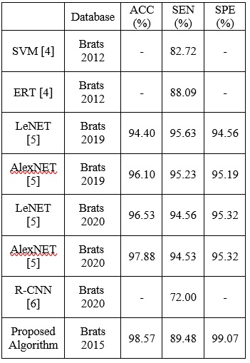
Soltaninejad et al. [4] proposed a fully automated algorithm to identify abnormal tissues in the brain based on super pixel technology and classify each pixel according to the characteristics extracted from it using the Extremely Randomized Trees (ERT) classifier. The researchers used two databases that were diagnosed as tumors. Glioma of varying degrees, the first database from the Health Care Center (General Electric GE) in the United States of America: 19 images in which the degree of glioma varies from the second to the fourth degree, the second database from the BRATS 2012 website, the number of 30 images, 10 of tumors Grade I and II gliomas, 20 for grade III and IV gliomas. The researchers compared the results of the ERT classifier and the results of the Support Vector Machine SVM in terms of precision and sensitivity for both rules. For the first rule, the results of precision and sensitivity of the ERT classifier were 87.86% and 89.48%, respectively, and the results of the accuracy and sensitivity of the SVM classifier were 83.59% and 87.82% respectively. As for the second rule, the results of the precision and sensitivity of the ERT classifier were 89.09%, 88.09%, respectively, and the results of the accuracy and sensitivity of the SVM classifier were 83.79%, 82.72%, respectively. We notice that the ERT classifier is better than the SVM classifier.
While Gomathi et al. [5] used two pre-trained deep learning models, namely the AlexNet model and the LeNet model. The two models were trained on the Brats 2019 database and the Brats 2020 database. The researchers compared the results of the AlexNet model with the results of the LeNet model in terms of accuracy, sensitivity, and specificity for both databases. For the Brats 2019 database, the accuracy, sensitivity, and specificity results of the AlexNet model were 96.10%, 95.23%, and 95.19%, respectively, and the accuracy, sensitivity, and specificity results of the LeNet model were 94.40%, 95.63%, and 94.56%, respectively, and for the Brats 2020 database, the accuracy results were The sensitivity and specificity of the AlexNet model are 97.88%, 94.53%, and 95.32%, respectively, and the results of the accuracy, sensitivity, and specificity of the LeNet model are 96.53%, 94.56%, and 95.32%, respectively. We notice that the AlexNet model is better than the LeNet model. Singh et al. [6] used Region Based Convolutional Neural Networks to train the ResNet model on Brats 2020 database and the results were as follows: F-scale 0.75, sensitivity 72%, precision 79%. |
|
| |
|
| 2. METHODOLOGY: |
|
Two databases of brain magnetic response images, consisting of approximately 1100 images, were obtained. The first database was 20 images, including 10 images diagnosed as benign brain tumors and 10 images diagnosed as malignant brain tumors of different dimensions [7]. The second database was from the BRATS 2015 website with a total number of 1080 slides from 108 patients 10 slides for each patient. 540 slides of them are diagnosed as benign brain tumors and 540 slides are diagnosed as malignant brain tumors with dimensions of 240 * 240 [8].
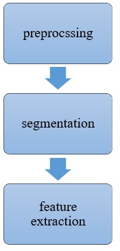
Our proposed methodology consists of 3 stages: preprocessing, Segmentation, and feature extraction. The flow chart of the proposed method is shown in Figure 1. |
|
| |
|
 |
|
| Fig. 1. Flowchart of the proposed method |
|
| |
|
| 2.1. Preprocessing: |
|
This stage consists of three main steps:
a) Convert RGB images to grayscale and then resize to 400*400 pixels
b) Remove the skull from MR images using morphological processes and pixel subtractions.
c) filtering of the image
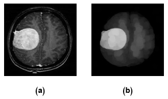
2.1.1. Remove the skull from MR images: In this study, the skull (bright region) of the image is extracted using an opening operation with the structure element “disk” and radius “13”. Figure (2) shows the result of applying the opening operation to the original image with the structure element “disk” and radius “13”. |
|
| |
|
 |
|
| Fig. 2. (a) Original Image. (b) Opened Image |
|
When the skull is removed, some of the pixels are also removed from the tumor region unintentionally. Therefore, an opened image can not be used directly for the tumor’s segmentation. The opening operation on its own is not enough to remove the skull properly. Pixel subtraction is used to extract the skull from the brain image in a more efficient manner.
Pixel subtraction: the following pixel subtraction operations are conducted.
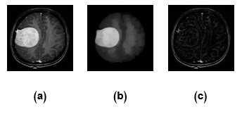
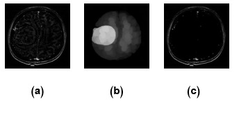
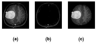
First, the image obtained from the opening operation is subtracted from the original image which separates the skull from the original image. Then the image obtained from the opening operation is subtracted from the skull image which removes the undesired gray pixels from the skull image. Lastly, the cleaned skull image is subtracted from the original image. The result of the pixel subtraction operations, the image of the brain is obtained without the skull. Figures (3,4 and 5) show the results of applying the Pixel subtraction Operations respectively. |
|
| |
|
 |
|
| Fig. 3. (a) Original Image. (b) Opened Image. (c) Skull Image |
|
| |
|
 |
|
| Fig. 4. (a) Skull Image. (b) Opened Image. (c) Cleaned Skull Image. |
|
| |
|
 |
|
| Fig. 5. (a) Original Image. (b) Cleaned Skull Image. (c) Skull Removed Image. |
|
| |
|
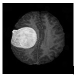
| 2.1.2. Filtering stage: The purpose of image filtering is to remove the noise on digital images. Image filtering is one of the most common issues in digital image processing. One of the most popular methods for image filtering is the median filter. In this filter, the median pixel value in the neighborhood is calculated and the middle pixel value in the neighborhood is replaced by the calculated median pixel value While calculating the median pixel value, all the pixel values in the neighborhood are first sorted in ascending order, and then the pixel values are evaluated together with the middle pixel value [9]. In this study, 3x3 neighborhood pixels around the evaluated pixel are used. Figure (6) shows the result of applying The median filter. |
|
| |
|
 |
|
| Fig. 6. Filtered Image |
|
| |
|
| 2.2. Segmentation: |
|
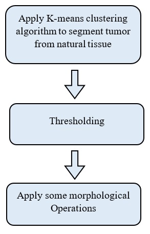
| The primary goal of the segmentation stage is to automatically separate the tumor from the background with the highest possible accuracy, by applying the K means clustering algorithm and then thresholding the image and applying some morphological operation to get the region of interest ROI. Figure 8 shows the flow chart: |
|
| |
|
 |
|
| Fig. 7. Flowchart of the proposed method |
|
| |
|
| 2.2.1. K means clustering: |
|
Looking at the image resulting from the previous stage as groups of data in which each group is similar in gray levels, therefore, the K means clustering algorithm can be used to segment the image into groups, and the group in which the mean value is higher is the group that represents the tumor. In the proposed algorithm, the number of clusters K is chosen to be 2 according to the following steps:
1. Define the number of clusters ‘K’.
2. Randomly, define cluster centers ‘C’.
3. Calculate the distance between each data point and cluster centers.
4. Data point is assigned to the cluster center whose distance from the cluster center is the minimum of all the cluster centers.
5. Then, new cluster center is recalculated as follows. |
|
 |
|
where ‘C’i is the number of data points in i-th cluster.
6. Recalculate the distance between each data point and newly acquired cluster centers.
7. If no data point was reassigned then stop, otherwise repeat steps 3 to 6.
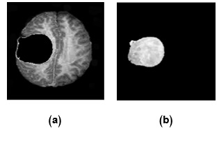
At the end of this stage, we get two images, the first representing the normal tissue of the brain, and the second representing the tumor, as shown in Figure (8): |
|
| |
|
 |
|
| Fig. 8. (a) Normal tissue of the brain. (b) Brain tumor. |
|
| |
|
| 2.2.2. Thresholding: Converting the image representing the brain tumor from a gray image to a binary image in which the tumor is white and the background and normal tissue are black, as shown in Figure (9): |
|
| |
|
 |
|
| Fig. 9. Binary Image |
|
| |
|
| 2.2.3. morphological operations: Apply the dilation operation with a disc element with a radius of 12 to merge the discontinuities and fill the holes, then apply the erosion operation with a disc element with a radius of 10 to remove small non-tumor areas to obtain a tumor mask, as shown in Figure (10): |
|
| |
|
 |
|
| Fig. 10. Tumor Mask |
|
| 2.3. Feature extraction: |
|
After the completion of the image segmentation stage, shapes’ features are performed on the segmented objects or regions in the image. For each shape in the binary image, the Matlab function ‘regionprops’ has a number of properties. In this paper, two shape properties were used including Area and Centroid. Descriptions of these features are given below:
Area: The area of the object is calculated using the actual total number of pixels which are present inside the object, which describes the area of that region.
Centroid: Center of mass of the region. returned as a 1-by-Q vector. The first element of Centroid is the horizontal coordinate (or x-coordinate) of the center of mass. The second element is the vertical coordinate (or y-coordinate). |
|
| 2.3.1. Tumor area as a percentage: |
|
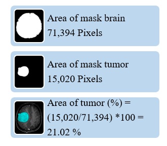
A special algorithm was developed to calculate the tumor area in percentage according to the following steps:
1. Thresholding the image resulting from the preprocessing stage, which represents only normal tissue and tumor (the brain mask), as shown in Figure (11), and calculating the area. |
|
| |
|
 |
|
| Fig. 11. Brain Mask |
|
| |
|
2. Calculation of the tumor area from the tumor mask shown in Figure (10).
3. Calculating the tumor area in percentage: using the following equation:
Tumor area in percent = (area of the tumor / area of the brain mask) * 100
Figure (12) shows the flowchart for calculating the tumor area in percentage: |
|
| |
|
 |
|
| Fig. 12. Flowchart for calculating the tumor area in percentage |
|
| |
|
| 2.4. Graphical User Interface: |
|
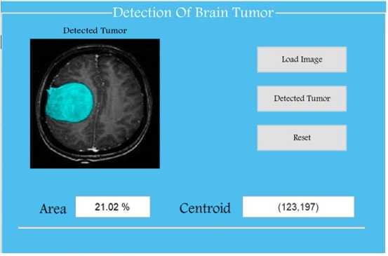
A very simple software interface was designed using Matlab software. In it, the tumor is identified on the image, its area is calculated in percentage, and its coordinates are determined. The interface includes only three commands, as shown in Figure (13):
Command (Load Image): to load the image.
Command (Detected Tumor): To mark the tumor on the image in blue and show its area in percentage in the Area text box and its coordinates in the Centroid text box.
Command (Reset): To delete all writing fields and the displayed image, and return the interface to its first operating position. |
|
| |
|
 |
|
| Fig. 13. The graphical user interface |
|
| |
|
| 3. Results and discussion: |
|
The result of the tumor segmentation (Mask Tumor) was compared with the Ground Truth and a set of parameters were calculated for each image (TP, TN, FP, FN):
True Positive: The pixel is classified as a brain tumor and is true.
True Negative: The pixel is classified as a normal tissue or black background and is true.
False Positive: The pixel is classified as a brain tumor and is false.
False Negative: The pixel is classified as normal tissue or black background and is false.
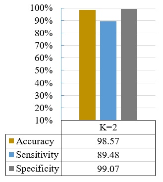
Accuracy, sensitivity, and specificity are calculated from these parameters, and then an mean is calculated for all database images to evaluate the performance of the proposed algorithm.
Accuracy = (TP+TN)/(TP+TN+FP+FN)
Sensitivity = TP/(TP+FN)
Specificity = TN/(TN+FP)
And when calculating the mean of all database images, results of accuracy, sensitivity, and specificity were shown in Figure (14). |
|
| |
|
 |
|
| Figure (14) Evaluation of the segmentation algorithm |
|
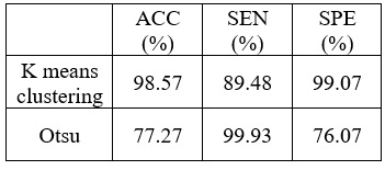
| A comparison was also made with Otsu thresholding, and this method aims to set an adaptive threshold value of intensity T(threshold) for every pixel such as each pixel is either categorized as a background point or an object point [10]. The accuracy results were 98.57% and 77.27% respectively, the sensitivity results were 89.48% and 99.93% respectively, and the specificity results were 99.07% and 76.07% respectively. The K means clustering algorithm showed the best results in terms of accuracy and specificity, while in sensitivity, the Otsu threshold showed better results due to the increase in the number of white pixels in the image because the adaptive threshold in the Otsu method led to the complete separation of the brain from the background and not the separation of the tumor from the normal tissue. |
|
| |
|
| Table 1: Evaluation of segmentation between the Otsu threshold and K means clustering |
|
 |
|
| |
|
| Table (2) shows the results of the comparison between three reference studies with the results of the research in terms of the methods used in brain tumor segmentation, as the methods varied between machine learning and deep learning. |
|
| |
|
| Table (2): Evaluation of research results with previous studies |
|
 |
|
| |
|
| We note that the AlexNet model in [5] achieved the highest accuracy of 97.88%, while the specificity was equal to 95.32% with the LeNet model, and the LeNet model was superior in sensitivity to 95.63%. The proposed algorithm, based on the K means clustering algorithm, gave a better performance than previous studies in terms of accuracy and specificity. |
|
| |
|
| 4. Conclusions: |
|
| Image processing has become one of the most important sciences today. Today, image processing applications are used in many fields, including the medical field. Detecting a brain tumor in its early stages and accurately determining its size and location leads to higher accuracy in classifying the type of tumor. This work can be expanded by classifying the type of tumor if it is benign or malignant, and the proposed algorithm can also be developed to build the brain in a three-dimensional way to show the tumor completely and calculate its true size. |
|
| |
|
| References |
|
1. Young, R. M., Jamshidi, A., Davis, G., & Sherman, J. H. (2015). Current trends in the surgical management and treatment of adult glioblastoma. Annals of Translational Medicine. Vol. 3. No. 9. P: 15.
2. Umar, A. A., & Atabo, S. M. (2019). A review of imaging techniques in scientific research/clinical diagnosis. MOJ Anatomy & Physiology. Vol. 6. No. 5. P-p: 175–183. MedCrave Publishing.
3. Almutrafi, A., Bashawry, Y., AlShakweer, W., Al-Harbi, M., Altwairgi, A., & Al-Dandan, S. (2020). The Epidemiology of Primary Central Nervous System Tumors at the National Neurologic Institute in Saudi Arabia: A Ten-Year Single-Institution Study. Journal of Cancer Epidemiology. Vol. 2020. P: 9. Hindawi.
4. Soltaninejad, Mohammadreza, Yang, Guang, Lambrou, Tryphon, Allinson, Nigel, Jones, Timothy L., Barrick, Thomas R., Howe, Franklyn A., & Ye, Xujiong. (2017). Automated brain tumour detection and segmentation using superpixel-based extremely randomized trees in FLAIR MRI. International Journal of Computer Assisted Radiology and Surgery. Vol. 12. No. 2. P-p: 183–203.
5. Gomathi, M., & Dhanasekaran, D. (2022). Glioma Detection and Segmentation Using Deep Learning Architectures. Mathematical Statistician and Engineering Applications. Vol. 71. No. 4. pp: 452–461.
6. Singh, Sanskriti. (2022). A Novel Mask R-CNN Model to Segment Heterogeneous Brain Tumors through Image Subtraction. arXiv Preprint. arXiv:2204.01201.
7. https://github.com/yashpasar/Brain-Tumor-Classification-and-Detection-Machine-Learning
(accessed 1/Sep/2021)
8. https://www.kaggle.com/datasets/andrewmvd/brain-tumor-segmentation-in-mri-brats-2015.
(accessed 1/May/2021)
9. Ammar, Maan. (2014). Medical image display and processing systems. Damascus: Syria. Damascus University Publications. P: 400. (in Arabic).
10. Otsu, N. (1979). A Threshold Selection Method from Gray-Level Histograms. IEEE Transactions on Systems, Man, and Cybernetics. Vol. 9. No. 1. p-p: 62–66. |
|
| |
|
| |
|
| |
|
|